Classification에서는 Linear Regression을 directly하게 사용할 수 없다
-> Classification은 discrete한 output인 반면에 Linear Regression의 ouput은 어떤 수치값이며 연속적이라 discrete 하지 않기때문에
-> 따라서 Linear Regression function에 뭔가 조작이 필요
-> 이래서 등장한 게 Logistic Regression!
Logistic Regression
linear regression model을 sigmoid function에 넣은 형태 ( sigmoid는 output이 항상 0~1 사이이기에 classification을 도와준다 )
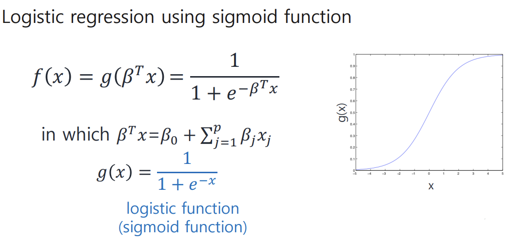
sigmoid function 선택하면 좋은 점 : g(x)를 미분취하면 final output이 g(x)를 사용한 form으로 떨어져서

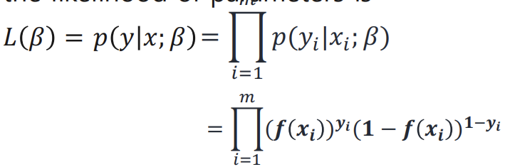
:likelihood를 maximize 하는 게 목표 ( 각 샘플의 등장 확률을 maximize )
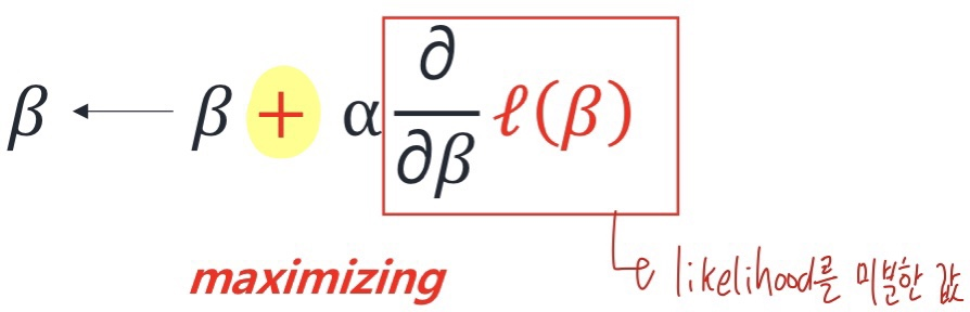
parameter 찾는 방법 : logistic regression은 likelihood를 높이는 방향으로 parameter optimization 한다.
-> likelihood를 maximize 하기 위해서 Gradient Ascent 사용한다 (왜 ascent? likelihood를 높이는 방향으로 parameter 찾아야해서)
Gradient Ascent
: iterative optimization algorithm for finding local maxima of a function

Logistic Regression 과정/알고리즘
1. Fit parameters
: find good parameters maximizing the likelihood of function ( use gradient ascent )
2. Predict on testing datapoint x'
:P(y=1|x';b)=f(x') / P(y=0|x';b)=f(x')
Gradient descent처럼 multiple iteration 쓰는 건 여러번 해야해서 비쌀 수 있다. 더 빨리할 수 있는 방법 없을까?!
-> Newton's method
Newton's method
-> 주어진 함수 값을 0으로 만드는 값 찾는 게 목표

장점 : fast convergence (0으로 가는 값을 더 빨리 찾을 수 있다)
단점 : inefficient ( inverting Hessian matrix가 비쌈)

Discriminative learning algorithm
: 관찰하려는 값의 확률을 직접적으로 decision boundary를 찾아서 어디에 더 해당되는지 구함
: 클래스 간의 결정경계를 이해하는데 관심
Generative learning algorithm
: 각 class에 해당하는 모델을 먼저 정의하고, 정의한 상태에서 각 sample의 probability 값을 구하는 방식
: 각기 다른 class에 대해 모델을 정의하는 데 집중한다.
: not directly compute p(y|x) instead, compute it through the likelihood (p(x|y)) and the prior (p(y))
: bayes rule 이용하여 확률 계산
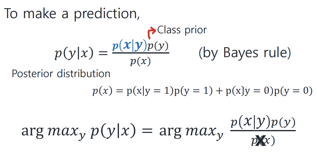
-> 위 사진에서 argmax인 이유 : 어떤 모델에 나타나는 확률이 큰 지 알아내야되는거라서
: posterior probability = (likelihood * prior)/p(x)
-> posterior probability = 실험 진행 후 관측하는 데이터가 y일 확률
-> likelihood = 실험을 통해 얻어지는 값으로 어떤 모델에서 해당 데이터가 나올 확률
-> prior = 실험 전부터 모델이 갖고 있는 확률
: 예시 중 GDA (Gaussian discriminant analysis) 존재
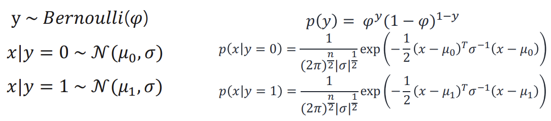
GDA
-> 얘는 p(x|y) 는 multivariate normal distribution을 따른다고 가정할 때 사용 가능

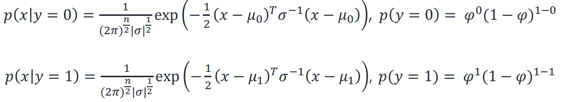
p(y),p(x|y=0), p(x|y=1) 수식은 다음과 같다
< Loglikelihood of GDA 수행 과정 >
Step 1. Compute MLE of parameters ( mean, covariance on each class & phi )

Step 2. Compute likelihood of each sample & prior (p(x|y=1), p(x|y=0), p(y)) using params computed in Step1
Step3. Compute posterior probability

GDA vs Logistic Regression
- p(x|y) 가 gaussian distribution을 따른다고 가정되면 GDA 사용하는 게 좋다!
-> Why? : iteration없고 mean과 covariance만 계산하면 됨
- 저런 가정이 없다면 Logistic Regression 사용하기 ( 이 모델이 덜 민감해서 )
->실제로 Logistic Regression이ger 더 많이 쓰인다
Naive Bayes (GDA와 비슷한 방법)
- text classification에 효과적인 classification 방법이다
- 동작 원리
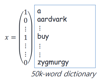
1. construct feature vector x ( 5000개의 사전에 있는 word를 쭉 봐서 해당 단어 나타났으면 1, 안 나타났으면 0. 이런식으로 feature vector를 각각의 email 마다 구성 )
-> 여기에 discriminative algorithm 적용하면 parameter가 (2**5000-1) 개 -> parameter가 너무 많다!!
-> 따라서 Generative algorithm 사용하자
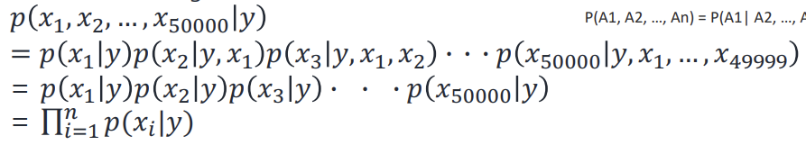
-> p(x|y) 모델을 만들기 위해서 xi's 들은 conditionally independent given y 라는 assumption이 있어야 Naive Bayes classifier 적용가능( 각각의 word는 conditionally independent하다 )
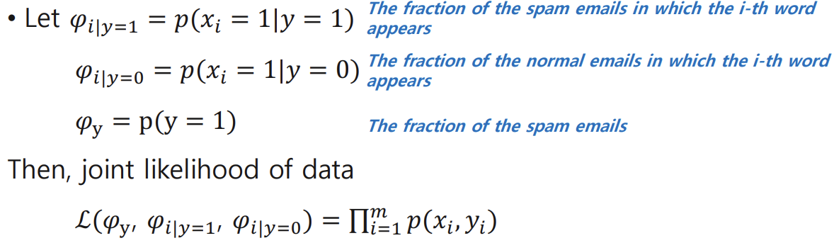
< Naive Bayes 과정>
1. Find the likelihood of each word being produced from spam or normal emails and the prior.
2. Compute the posterior probabilities for each class.
3. Pick the class with the highest probability

Laplace smoothing
0/0꼴 해결방법
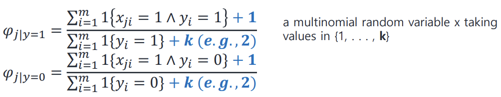
k : x가 될 수 있는 개수
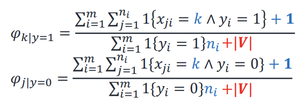
Multinomial event model
-> 사전 속 단어 하나하나가 출현했는지 표현하는 게 아니라 이메일 본 후 단어 index로 feature vector 만드는 방법
( feature 길이 = 단어 개수)

cf) ml_lec_06 시작 부분 요약 + naive bayes 예제 다시 풀어보기
'인공지능 > Machine Learning' 카테고리의 다른 글
| model assessment (0) | 2023.12.11 |
|---|---|
| Decision tree (0) | 2023.10.26 |
| Soft margin classifier (0) | 2023.10.25 |
| SVM (Hard margin classifier) (0) | 2023.10.24 |
| Linear Regression(2) (1) | 2023.10.22 |


